Imagine you are designing a system where there would be 100k writes/sec. Using Postgres or MySQL to store the events would be slow because under the hood, they use B-trees. B-trees maintain data in sorted order. So every write has to land at a specific position in the tree. This means each write is essentially a random I/O operation (you have to seek to the right leaf page on disk). Random I/O is significantly slower than sequential I/O, even on SSDs. Moreover, when a leaf page fills up, it has to split and the parent node has to be updated to point to the new pages. This can cascade up the tree, causing multiple disk writes for what was a single logical write. Enough about B trees for now, I’ll cover B-trees in detail in a future blog.
I can hear you saying, why not do event streaming? Well, the answer is simple. Event streaming systems like Kafka improve write throughput using log-structured storage, but they don’t replace the need for an efficient storage engine underneath. The problem at the storage layer still remains. The write latency is still there. So, what can we do to reduce the write latency? Instead of propagating the writes to the leaf nodes, as we do in B-trees, can’t we simply append the data sequentially as we receive it? This is exactly what Log structured storages do.
Log Structured Storages
Let’s first describe a very simplistic Log structured storage. As we mentioned before, we don’t complicate writes. We just append the data sequentially as we receive it. Now the problem is how do we read the data? We can simply read the data in the order it was written. But this is not efficient. And writing data to disk one by one is slow even for sequential writes. So, how about we store it in memory?
Now the writes are fast, but reading is still a problem. Let’s introduce an index to help us know the address of the key of the data we are looking for. Let’s have a hashmap to store the key of the data and the address of the data (offset - distance from the start of the file - Now we know the starting point of the data we want instead of searching from the beginning) as key value pairs. Now, when we want to read the data, we can simply look up the key in the hashmap and get the offset. This approach is good if you have a huge amount of memory. But practically, the memory alone is not sufficient especially if there are huge amount of keys or you need to store multicolumn values for each key. So what if we keep flushing the data to disk sequentially as and when the memory is full?
SSTables
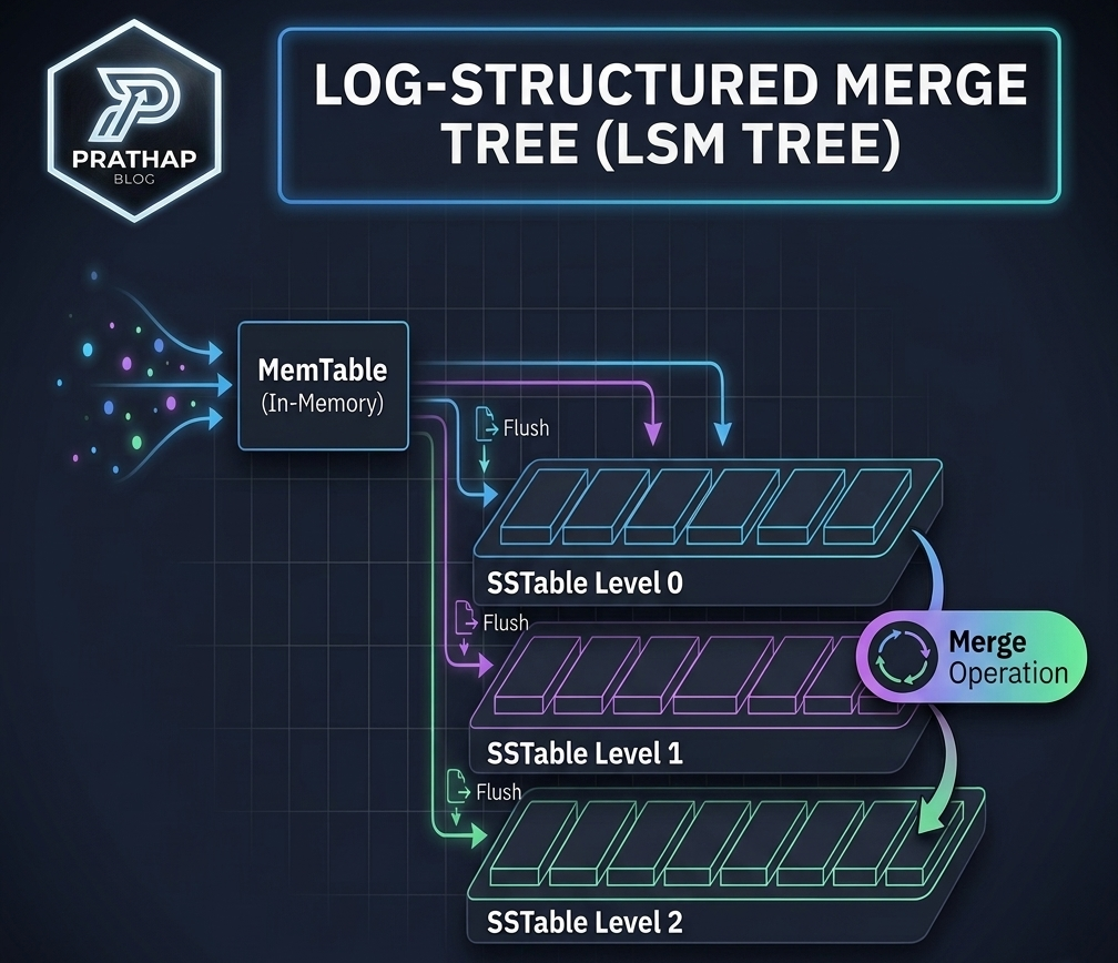
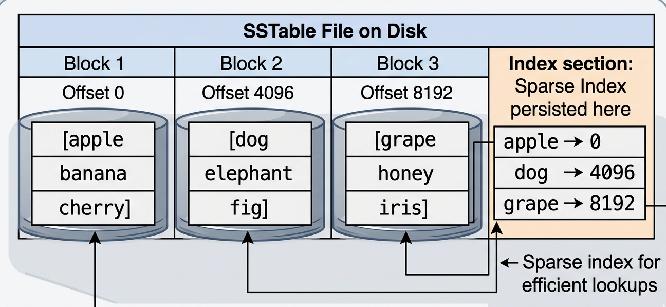
But how can one accomplish this? First replace the hashmap with a searchable data structure like a simple Binary Search Tree (Note - actual implementation uses a self balancing tree like red-black tree). We will call this the Memtable. Now when the memtable is full or reaches a pre-defined size, we will start writing sequentially to the disk in small blocks of a fixed size. We start inorder traversal of the memtable and write the data sequentially to the disk until we reach a fixed size, mark it as a block. We also keep the first key of the block and the offset of the block in an index. The method of storing just the start of the block is called sparse indexing. This process will keep continuing until all the keys in the memtable are flushed to disk and the memory occupied by the memtable will be returned. The index along with the blocks will be stored in a file called SSTable. SSTable means Sorted String Table. As you know we traverse the memtable in inorder fashion, so the keys in the SSTable will be sorted. Hence the name Sorted String Table. This flushing process will keep happening in the background while the new memtable is receiving new writes. This happens every time the memtable reaches a certain size or when it is full. As a result, there will be a lot of SSTables.
A lot of SSTables is a problem in the read path. To understand this, let’s see how a key is read. We’ll keep things simple. Let’s assume there are no blocks in the SSTables, no sparse index. Just the key and the value. First, we will check if the memtable has the key. If not, we will check the SSTables. We will start traversing the SSTables from the most recent one to the oldest one. This is the problem in the read path. Traversing the individual SSTables is not a slow process. Because the SSTables are sorted (remember how we flush the memtable we do inorder traversal), so the search is O(log n). But traversing through all the SSTables on the disk from recent to oldest until you get your key is slow. This can be helped to a certain extent by attaching a bloom filter for each SSTable to reduce unnecessary disk reads. We’ll deep dive into bloom filters in a future blog, but for now let’s look at how bloom filters can help us.
A bloom filter can definitively tell you if a key is not in an SSTable. So you can skip it without touching the disk. But some of the bloom filters will return false positives, claiming the key might be there when it isn’t, and you end up reading that SSTable from the disk. So to read an amount of bytes of data (the data that you want), you end up reading a huge amount of data to get to the correct SSTable (the SSTables before reaching the correct SSTable). This is called Read Amplification So, how can we solve this?
Before getting into it, let’s get a picture of what gets into the SSTables, when we keep writing keys that are not new. Let’s say we write a key “Armour” with value “9000”. As we know, this will be written to the memtable. Let’s say the memtable is flushed to the disk and we write the key “Armour” again with value “10000”. Now the memtable and the SSTable will have the same key “Armour”. As a result, if we keep writing “Armour” to the DB, many SSTables will have the same key. So which key value pair should be considered on read path? The latest one. First the memtable and then the most recent SSTable - this is the reason why we traverse the SSTables from most recent to the oldest one. As you can see, there will be a lot of duplicate key value pairs in the SSTables. This can be one of the reasons for having a large number of SSTables. Since there are duplicate key value pairs, can we remove the duplicate key value pairs and keep just the latest one? This is done by a process called Compaction.
Before going into the details of compaction, let’s see how the memtable is flushed to the disk. Here is a simulation of how the memtable is filled and then flushed to the disk. On the control panel, you can either write a randomly generated key-value pair or write a key-value pair manually. There is a search button to search for a key. The search will start from the memtable and then move to the SSTables. The component that is being searched will flash. If the key is found, the key-value pair will be highlighted. Try giving it a spin.
LSM Tree — Write & Search Simulation
Compaction
As we understood earlier, a large number of SSTables is bad for read path. And we also know the reason for this - the duplicate key value pairs. If a key is in four SSTables, why don’t we just keep the latest one? This is what compaction does. When a threshold number of SSTables is reached or when a similar threshold is reached - depending on the type of compaction configured, the compaction process starts. In general the compaction process is simple, it is just n-way mergesort of the SSTables.
So far we have seen writing/updating or reading a key. But what about deleting a key? When the key is to be deleted, a special marker is written against the key to be deleted. This marker is called tombstone. Just like how the duplicate keys are removed, the tombstone is also removed during the compaction process.
Here is a simulation that shows how 4 SSTables are merged into 1 SSTable. Click on generate to populate the SSTables. Click on step to see how the SSTables are compacted. There will be 4 cursors, each pointing to a SSTable. The cursors will flash as the mergesort progresses. At each step, the candidate cursors for pushing into the new SSTable flashe in purple. The winner cursor flashes in green. The candidates are the cursors that have the minimum key. The winner is the latest cursor that has the minimum key and that is written to the new SSTable. If the winner is a tombstone, the key is deleted and the older version is discarded.
Click on generate to populate the SSTables with random values. Then click on Step to see the candidates that were considered and which was the winning candidate for the merge. See it getting inserted into the latest SSTable. Try giving it a spin.
Now, compaction sounds simple. But there is still an important question. Which SSTables do you compact? And when? The answer to this is the compaction strategy. There are two main compaction strategies: Size Tiered Compaction and Leveled Compaction.
Size Tiered Compaction
Think of Size Tiered Compaction (STCS) as a sorting hat that groups SSTables by size. Every time the memtable is flushed, a small SSTable lands on disk. Once you have enough small SSTables of roughly the same size (usally 4), they are merged into a single larger SSTable. That larger SSTable now sits alongside other large SSTables. Once enough large SSTables accumulate, they too are merged into an even larger one. And so on. The resulting structure looks like a set of tiers. Tier 1 has the smallest and newest SSTables. Tier 2 has the next size up. And so on. Each tier is roughly 10x the size of the previous one.
Okay now let’s unpack this. With this approach, number of times you have to compact is small because as you go up the tiers, the number of keys in each SSTable is bigger, so the time taken to reach the threshold is bigger. Hence the total number of compactions is small. This is a good time to introduce Write Amplification. Just like read amplification, to write an amount of bytes of data (the data that you want to write), you end up writing it multiple times - since you keep merging SSTables, you end up writing the same data multiple times. This is write Amplification.
We kept the number of merges to a minimum by merging SSTables in size order. But there is a problem. Let’s explain it with an example.
Let’s say we have 4 tier 0 SSTables. Each tier 0 SSTable is formed by flushing the memtable.
Flush 1 → SSTable A (tier 0): [apple, banana, cherry]
Flush 2 → SSTable B (tier 0): [banana, date, elderberry]
Flush 3 → SSTable C (tier 0): [apple, cherry, fig]
Flush 4 → SSTable D (tier 0): [date, grape, kiwi]
Now we have reached the threshold of 4 SSTables. We need to merge them into a single SSTable. Let’s say we merge SSTables A, B, C, D into SSTable E.
Merge 1 → SSTable E (tier 1): [apple, banana, cherry, date, elderberry, fig, grape, kiwi]
Now you keep writing, get 4 more flushes, and tier 1 fills up again. So you merge SSTables and create SSTable F.
Merge 2 → SSTable F (tier 1) [avocado, banana, cherry, durian, elderberry, fig, guava, lemon]
Look at tier 1. SSTable E covers (apple → kiwi) and SSTable F covers (avocado → lemon). They overlap heavily. Meaning, if you want to read a key that starts with “a”, you have to check both SSTables. This is a problem that we have already seen - Read Amplification.
From what we have seen, STCS is a good fit when your workload is write-heavy (write is easy because lesser compaction merges) and you can tolerate slightly slower reads (read is slow because of the overlapping ranges). Cassandra used to have STCS as its default compaction strategy.
Leveled Compaction
Leveled Compaction (LCS) takes a stricter approach. Instead of grouping by size, it organises SSTables into fixed levels. Level 0 (L0) is where the freshly flushed memtables land. The critical rule in LCS is that within any given level except L0, no two SSTables can have overlapping key ranges. So when you read, you just check exactly one SSTable per level.
The main difference between STCS and LCS is that in LCS, we take care of the overlapping ranges during the write/merge phase so that read path latency is predictable. This is the trade-off we make.
Ok bear with me now as I take you through LCS with a simple but long example.
Like earlier example, we have 4 tier 0 SSTables formed by flushing the memtable.
Flush 1 → SSTable A (L0): [apple, banana, cherry]
Flush 2 → SSTable B (L0): [banana, date, elderberry]
Flush 3 → SSTable C (L0): [apple, cherry, fig]
Flush 4 → SSTable D (L0): [date, grape, kiwi]
Now we reached the threshold of 4 SSTables. We need to merge them into a single SSTable. Since we need to take care of the overlapping during merge, we first create a stream of input where we use the same method that we followed in STCS. We’ll have a cursor for each SSTable. We identify the candidates and add the winner to the stream.
So now we get this stream → [apple, banana, cherry, date, elderberry, fig, grape, kiwi]
Now we create L1 SSTables from this stream. As always we have a size limit for each block. So we start with the first key in the stream and fill the first block and then we start filling the next block.
So now we get these L1 SSTables:
Merge 1 → SSTable E (L1): [apple, banana, cherry, date] SSTable F (L1): [elderberry, fig, grape, kiwi]
L1 at this point is clean. E and F have non-overlapping key ranges, which is the key rule of LCS.
Let’s say we get more flushes from the memtable.
Flush 5 → SSTable G (L0): [banana, cherry, fig]
Flush 6 → SSTable H (L0): [apple, date, guava]
Flush 7 → SSTable I (L0): [cherry, fig, lemon]
Flush 8 → SSTable J (L0): [banana, mango, fig]
Like earlier, we get the input stream from the L0 SSTables → [apple, banana, cherry, date, fig, guava, lemon, mango]
Now before we can write these into L1, we need to check which existing L1 SSTables overlap with this stream’s key range. The stream spans from apple to mango, which overlaps with both E (apple to date) and F (elderberry to kiwi). So we must pull E and F out of L1 and merge them together with the incoming stream.
The combined input stream is now → [apple, banana, cherry, date, elderberry, fig, grape, guava, kiwi, lemon, mango]
We split this into new L1 SSTables:
Merge 2 → SSTable E (L1): [apple, banana, cherry, date, elderberry] SSTable F (L1): [fig, grape, guava, kiwi, lemon, mango]
As you can see there are no overlaps anywhere in L1. In this example, we saw the L1 SSTables getting created. But as the system grows, there will be a time when the L0 SSTables need to be merged with existing L1 SSTables. The rule of thumb is to pick one SSTable from level L and merge it with SSTables in level L+1 which overlaps with the key range of the level L SSTable.
From what we have seen, LCS is a good fit when your workload is read-heavy (reads are fast because each level maintains non-overlapping key ranges, so any key can be found in exactly one SSTable per level) and you can tolerate higher write costs (writes are expensive because a single flush can cascade compactions down multiple levels, causing high write amplification). RocksDB uses LCS as its default compaction strategy.
The trade-off
The choice between STCS and LCS is ultimately a trade-off between write amplification and read amplification. STCS is cheaper to write to but more expensive to read from. LCS is more expensive to write to but cheaper to read from. Most production systems expose both as configuration options and let you choose based on your workload.
Conclusion
From this read, I hope you can now understand why Cassandra is used for systems with high write throughput like IoT sensors data streaming, user click events etc. We have just seen the high level implementation of LSM trees and how they are used to achieve high write throughput. But there is more to it. For example, we haven’t covered the durability of LSM trees. And if you notice, the systems in our example are just key value stores and not multi column records. I’ll leave you with interesting problem. What happens when the memtable fills up faster than compaction can keep up?
I hope I have done justice to your time reading this. See you in the next blog.
Cheers. 💛